Anscombe's quartet and monitoring
Anscombe’s quartet is a collection of four data sets of points in the plane. When graphed the data sets are obviously very different, but they have identical sets of descriptive statistics. Newer variations on the same theme include the delightful Datasaurus dozen, which includes animations of deformations from one step into another where the descriptive statistics are kept identical during the animation.
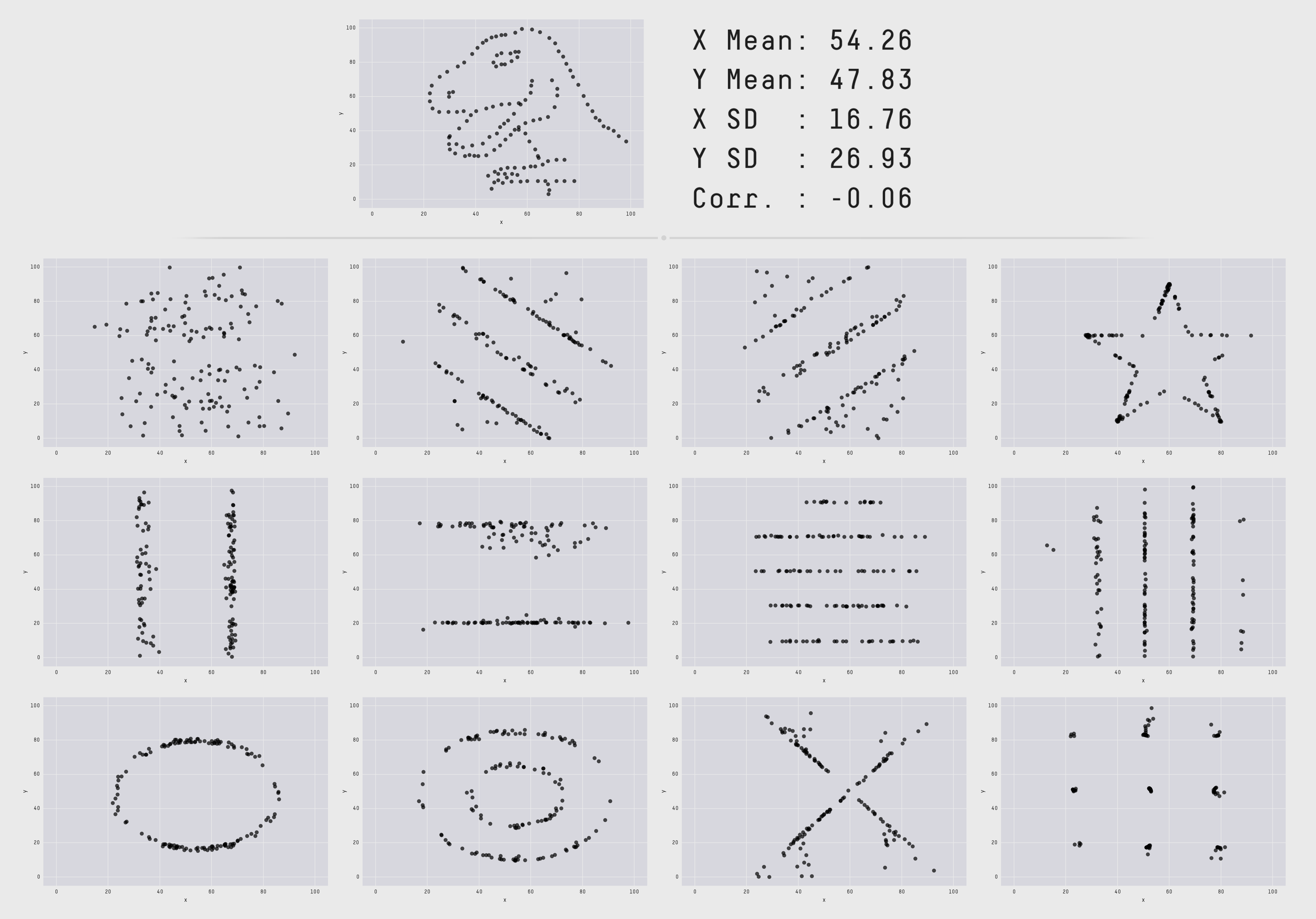
I’ve seen Anscombe’s quartet cited in discussions around monitoring and observability to assert that the average and standard deviation (two of the statistical tools used in the quartet) are not useful for monitoring and alerting; instead one should use percentiles. I agree with the conclusion but think it does not follow from the premise, and would like to offer some thoughts on the theme from the perspective of a reformed geometer.
To do so, I’d like to work out some examples involving the average and standard deviation. The data sets above involve collections of points in the plane but I’d like us to discuss data modeled on timeseries instead. The difference isn’t important, everything we say applies to both theaters, but the geometry we want to point out is easier to see in the latter.
Setup
We’ll model a portion of a timeseries as a tuple of \(n\) real numbers \((x_1, \ldots, x_n)\). We can think of these as \(n\) measurements recorded at one-second (or minute, hour, …) intervals. The set of all possible such timeseries is familiar; it is the real vector space \(\mathbb{R}^n\) of dimension \(n\). (Timeseries can be added and subtracted, there is a zero-timeseries that serves as an identity, and we can multiply a timeseries by a real number.)
The main characters of our story are the average and standard deviation. If \(x = (x_1, \ldots, x_n)\) is a timeseries, its average is \[ \mu(x) = (x_1 + \cdots + x_n) / n \] and its standard deviation is defined by the scary formula[1] \[ \sigma(x) = \sqrt{ ( (x_1 - \mu(x) )^2 + \cdots + (x_n - \mu(x) )^2 ) / n }. \]
We can now look at some examples. In every one of these, we’ll fix the average and standard deviation to some values and look at the collection of timeseries that have those values. The first couple of examples are just warm-up.
n = 1
We first look at \(n = 1\), that is, timeseries that just have one value \(x = (x_1)\). For such a timeseries we have \(\mu(x) = x_1\) and \(\sigma(x) = 0\) so each timeseries is uniquely determined by its average and they all have the same standard deviation.
n = 2
The next case is \(n = 2\), of timeseries with two values \(x = (x_1, x_2)\). This is slightly more interesting; we have the average \(\mu(x) = (x_1 + x_2) / 2\) and the standard deviation \[ \begin{align} \sigma(x) &= \sqrt{( (x_1 - \mu(x) )^2 + (x_2 - \mu(x) )^2 )/2} \\ &= \sqrt{((x_1 - x_2)^2 + (x_2 - x_1)^2)/8} = |x_1 - x_2|/2. \end{align} \] The second equality here is by substituting the definition of \(\mu(x)\).
This is more interesting because different timeseries can have different averages and standard deviations. However, I claim that if we fix both the values of the average and standard deviations, say to \(\mu\) and \(\sigma\), there is at most one timeseries that has those values.
To see this, observe that the formula for the average implies that \(x_2 = 2 \mu - x_1\), so if we fix the value of the average the value of \(x_2\) is determined by the choice of \(x_1\). If we substitute this into the formula for the standard deviation we get \[ \sigma(x) = |x_1 - 2 \mu + x_1|/2 = |x_1 - \mu|. \] We can solve this equation by splitting into cases where \(x_1 > \mu\) and \(x_1 < \mu\). In the former we get \(x_1 = \sigma + \mu\) and in the latter we get \(x_1 = \mu - \sigma\). Notice that in both cases, the value of \(x_1\) is determined by the values of the average and standard deviations, and the value of \(x_2\) is determined by that of \(x_1\) and the average, so both \(x_1\) and \(x_2\) are determined once we fix the others.
n = 3
We now get into the first case that has a hint of the general picture. Our timeseries have three points, \(x = (x_1, x_2, x_3)\). We could write down equations like in the previous case and calculate, but it’s worth it to take a step back and think about what’s going on.
Let’s say we have fixed the value of the average of our timeseries to a constant \(\mu\). The formula for the standard deviation of our series is then \[ \sigma(x) = \sqrt{((x_1 - \mu)^2 + (x_2 - \mu)^2 + (x_3 - \mu)^2)/2}. \] If we form the point \((\mu, \mu, \mu)\), we see that \[ \sigma(x) = \|(x_1, x_2, x_3) - (\mu, \mu, \mu)\|/\sqrt{2} \] is just a multiple of the Euclidean distance between our timeseries and the fixed point \((\mu, \mu, \mu)\). If we also fix \(\sigma(x) = \sigma\), the set of points that satisfy this equation is \[ S := \{ (x_1, x_2, x_3) \mid \|(x_1, x_2, x_3) - (\mu, \mu, \mu)\| = \sqrt{2} \sigma \}. \] This should look familiar, it is the sphere whose center is \((\mu, \mu, \mu)\) and whose radius is \(\sqrt{2}\sigma\).
Similarly, the set of timeseries whose average is equal to \(\mu\) is \[ P := \{ (x_1, x_2, x_3) \mid (x_1 + x_2 + x_3)/2 = \mu \}. \] For those who know a little linear algebra, we can write the condition as being that \((x_1, x_2, x_3) \cdot (1, 1, 1) = 2 \mu\), that is, that the inner product with \((1, 1, 1)\) must be equal to \(2 \mu\). The set of points that satisfies such a condition is a plane; a flat two-dimensional space.
We’re interested in the set of points where both of these conditions are true, which is the intersection \(S \cap P\). We could work out what that is by calculation, but it’s easiest to visualize it. The intersection of a sphere and a plane in three dimensions is either empty (when they don’t meet), a single point (when the plane is tangent to the sphere), or a circle that lies on the sphere.
In three dimensions, if we pick our values for the average and standard deviations right, there is thus a whole circle of timeseries that have that average and standard deviation. They form a kind of Anscombe set.
Higher dimensions
In higher dimensions, basically the same thing happens as in dimension 3. The set of timeseries that have a fixed average is a hyperplane and the set of timeseries that have a fixed standard deviation and average is a sphere. Their intersection, when it is not empty or a single point, is not as easily described but it is a subspace of dimension \(n-2\). As \(n\) grows higher, this space grows as well, and in general the space of timeseries that have a fixed average and standard deviation is enormous.
Other prescriptive statistics
The final point I’d like to make, and one you’ll have to take my word for to some extent, is that there is nothing special about the average or standard deviation here. Very similar things will happen for every collection of statistical tools we pick.
Every statistical tool can be viewed as a function that takes a timeseries (or perhaps a couple of timeseries, which complicates things a little but not a lot) and returns a real number. These functions are very well behaved (continuous, differentiable, and so on).
Given a collection of such functions \(f_1, \ldots, f_k\) on the space of timeseries of \(n\) points, we can ask whether there is an Anscombe set of fixed values of these functions? That is, if we fix values \(y_1, \ldots, y_k\), can we say anything about the set \(\{x = (x_1, \ldots, x_n) \mid f_1(x) = y_1, \ldots, f_k(x) = y_k \}\)?
With some hand waving, we can actually say this: Fixing the value of a single tool \(f_j\) creates a hypersurface \(X_j = \{x \mid f_j(x) = y_j\}\) inside the space of timeseries, that is, a subspace of dimension one less than the ambient space. All timeseries in \(X_j\) will have the same value with respect to this tool. If the intersection of all of these \(X_1 \cap \cdots \cap X_k\) is not empty, it will generally be a subspace of dimension \(n - k\). If \(n\) is much bigger than \(k\), the dimension of this space, the space of timeseries that all have the same statistical values with respect to our tools, is enormous.
Making the hand waving precise and figuring out when this intersection will be non-empty is the domain of algebraic geometry over the real numbers. Saying anything at all about that is beyond our scope here.
Outro
I hope I have convinced you that the statement "the average and standard deviation are useless for monitoring because of Anscombe’s quartet" is not true. The moral of Anscombe’s quartet, which boils down to intersection theory in algebraic geometry, is that the space of data that fits any given collection of statistical instruments (including any collection of percentiles) is gigantic and we have to look at the data to make sense of it.
In general, percentiles are more valuable for analyzing performance or traffic data than the average and standard deviation. The reason is not Anscombe’s quartet, the robustness of percentiles, or anything to do with normal distributions, but that the average and standard deviation are fundamentally tools for answering the questions "what would this be if it were constant?" and "how far away is this from being constant?".[2] For performance and traffic analysis, we don’t care about either of those questions, but about peaks in demand and how we can handle them. We should pick tools that can help with that, but other tools have their place.