It is well-known that the curvature properties of Kähler metrics "flow downward". To give meaning to this statement, let us say that a tensor \( \alpha \) dominates a tensor \( \beta \) if any of the following implications hold: \begin{align*} \alpha > 0 &\implies \beta > 0, & \alpha &\geq 0 \implies \beta \geq 0, \\ \alpha < 0 &\implies \beta < 0, & \alpha &\leq 0 \implies \beta \leq 0. \end{align*} Strictly speaking we need to specify what it means for a tensor to be "positive" or "negative" for this to make sense. This is fairly clear for the tensors we’ll discuss here, except for the Kähler curvature tensor itself which we mean to be Griffiths positive (or negative).

If \( R \) is the curvature tensor of a Kähler metric, its various derived curvature tensors are the holomorphic sectional curvature \( H \), the Ricci tensor \( r \) and the scalar curvature \( s \). Then \( R \to H \to s \) and \( R \to r \to s \), where an arrow \( \alpha \to \beta \) means that \( \alpha \) dominates \( \beta \).

The witches of the field know that neither \( H \) nor \( r \) dominates the other. The best evidence for this seems to be indirect. We for example know that Hirzebruch surfaces (surfaces that are projective bundles over \( \mathbf{P}^1 \)) carry metrics with positive holomorphic sectional curvature, but carry no metric of positive Ricci curvature as their anticanonical bundle is not ample. There are some suggestive results in the negatively curved case though, where a compact Kähler manifold that carries a metric of negative holomorphic sectional curvature also carries a possibly different metric of negative Ricci curvature. We don’t know if these are the same metric. It would be nice if some easy local calculations said they were, but in this note we will see they don’t.

It is also folklore that all of the reverse relations in the diagram fail. Some do not hold by general considerations; for example Hirzebruch surfaces again carry a metric of positive holomorphic sectional curvature but not one of positive Griffiths curvature, for otherwise they would be \( \mathbf{P}^2 \) by Siu—​Yau’s solution of the Frankel conjecture and, lo, they are not.

We feel like it would be nice to see explicitly what doesn’t hold here. In this light reading note we work out local examples that show that the reverse of any known positivity implication fails. As other people have noted it would be nice to have compact examples of these failures but it is fairly difficult to get one’s hands on those. Suggestions are welcome.

Let \( V \) be a complex vector space of dimension \( n \), which we think of as the tangent space of a complex manifold at a given point. The curvature tensor \( R \) of a Hermitian metric on the manifold identifies with a Hermitian form \( q \) on \( V \otimes V \), defined by \[ R(x, \overline{y}, z, \overline{w}) = q(x \otimes z, \overline{y \otimes w}). \] If the metric is Kähler we get an additional symmetry \( R(x, \overline{y}, z, \overline{w}) = R(z, \overline{y}, x, \overline{w}) \) (and the ones induced by conjugating).

We write \( B(V) \) for the real vector space of Hermitian forms on \( V \). The curvature tensor of a Hermitian metric is then just a member of \( B(V \otimes V) \). We’ll call such an element an algebraic curvature tensor, and one that satisfies the symmetries of a Kähler curvature tensor an algebraic Kähler curvature tensor.

Proposition If \( R \) is an algebraic Kähler curvature tensor, then \( R \to H \to s \) and \( R \to r \to s \).

This is both well-known and mostly easily proved by taking traces in an orthonormal basis. The trickiest impliciation is to show that \( H \to s \). Berger gave the original proof by showing that \[ \frac{1}{\operatorname{Vol} S^{2n-1}} \int_{S^{2n-1}} \!\!\! H(v) \, d\sigma(v) = \frac{1}{\binom{n+1}{2}} s \] by writing \( v = \sum_{j=1}^n v_j e_j \) in an orthonormal basis \( (e_j) \), expanding the curvature tensor \( R(v, \bar v, v, \bar v) \), and integrating polynomials in \( v_j \) over the sphere. (The reader who wants to try their hand at this can see Folland’s paper on integrating polynomials over spheres for the last part.)

Let’s define \begin{align*} \mathcal{H}(V) &= \{ \text{germs of smooth Hermitian metrics on \( V \) at \( 0 \)} \}, \\ \mathcal{K}(V) &= \{ \text{germs of smooth Kähler metrics on \( V \) at \( 0 \)} \}. \end{align*} We just write \( \mathcal{H} \) if \( V \) is clear from context and will usually mean \( V = \mathbf{C}^n \). Note that \( \mathcal{K} \) and \( \mathcal{H} \) are only convex open cones in real vector spaces and not full subspaces. Evaluating the curvature tensor of a metric at \( 0 \) defines nonlinear maps and a commutative diagram \begin{align*} \mathcal{K} &\stackrel{\mathcal{R}}{\longrightarrow} B(\operatorname{Sym}^2 \mathbf{C}^n) \\ \downarrow & \qquad\qquad \downarrow \\ \mathcal{H} &\stackrel{\mathcal{R}}{\longrightarrow} B(\mathbf{C}^n \otimes \mathbf{C}^n). \end{align*} Both vertical arrows are of course injective. The horizonal arrows are neither injective nor surjective in general.

Let \( H \) be the matrix of a Hermitian metric \( h \) in a neighborhood around \( 0 \) in \( V \). The Chern connection of \( h \) is given by \( D^{1,0} = H^{-1}\partial H \) and its curvature form is \[ F = \tfrac i2 \bar\partial(H^{-1}\partial H) = - \tfrac i2 H^{-1} \bar\partial H \wedge H^{-1} \partial H - \tfrac i2 H^{-1} \partial \bar\partial H. \] The curvature tensor is then \( R(x,\overline{y}, z, \overline{w}) = h(F(x, \overline{y}) z, \overline{w}) \).

We can pick coordinates such that \( H = I_n \) at \( 0 \). If \( h \) is Kähler we can further get \( \partial H = 0 \) at \( 0 \). We will arrange this in our examples. We now restrict to \( V = \mathbf{C}^2 \).

Proposition. The image of \( \mathcal{K}(\mathbf{C}^2) \) in \( B(\mathbf{C}^2 \otimes \mathbf{C}^2) \) is the set of matrices of the form \[ \begin{pmatrix} x & a & a & c \\ \bar a & z & z & b \\ \bar a & z & z & b \\ \bar c & \bar b & \bar b & y \end{pmatrix} \] where \( x, y, z \in \mathbf{R} \), \( a, b, c \in \mathbf{C} \).

Proof: If \( h \) is a Hermitian metric on a neighborhood of \( 0 \) in \( \mathbf{C}^2 \) we can write it in matrix form as \[ H = \begin{pmatrix} a & c \\ \overline{c} & b \end{pmatrix}. \] After a change of coordinates, we can assume that \( H(0) = I_2 \). Assuming \( h \) is Kähler we can also arrange that \( \partial H(0) = 0 \). Then the matrix of the curvature tensor in the basis \( (\partial / \partial z \otimes \partial / \partial z, \partial / \partial z \otimes \partial / \partial w, \partial / \partial w \otimes \partial / \partial z, \partial / \partial w \otimes \partial / \partial w) \) is \[ R = \begin{pmatrix} a_{z \overline{z}} & \overline{c}_{z \overline{z}} & a_{z \overline{w}} & \overline{c}_{z \overline{w}} \\ c_{z \overline{z}} & b_{z \overline{z}} & c_{z \overline{w}} & b_{z \overline{w}} \\ a_{w \overline{z}} & \overline{c}_{w \overline{z}} & a_{w \overline{w}} & \overline{c}_{w \overline{w}} \\ c_{w \overline{z}} & b_{w \overline{z}} & c_{w \overline{w}} & b_{w \overline{w}} \end{pmatrix}. \] We’ve written, for example, \( a_{z \overline{w}} \) instead of \( \frac{\partial^2 a}{\partial z \partial \overline{w}} \). The metric \( h \) is Kähler, so we have \[ a_w = c_{z}, \quad a_{\overline{w}} = \overline{c}_{\overline{z}}, \quad b_z = \overline{c}_w, \quad b_{\overline{z}} = c_{\overline{w}}, \] and thus \[ c_{z \overline{z}} = a_{w \overline{z}}, \quad \overline{c}_{w \overline{w}} = b_{z \overline{w}}, \quad c_{z \overline{w}} = a_{w \overline{w}}, \quad \overline{c}_{w \overline{z}} = b_{z \overline{z}} \] Then we get \[ R = \begin{pmatrix} a_{z \overline{z}} & a_{z \overline{w}} & a_{z \overline{w}} & a_{w \overline{w}} \\ a_{w \overline{z}} & a_{w \overline{w}} & a_{w \overline{w}} & b_{z \overline{w}} \\ a_{w \overline{z}} & a_{w \overline{w}} & a_{w \overline{w}} & b_{z \overline{w}} \\ a_{w \overline{w}} & b_{w \overline{z}} & b_{w \overline{z}} & b_{w \overline{w}} \end{pmatrix}, \] where some simplifications happen because \( a \) is real so \( a_{w \overline{z}} = a_{z \overline{w}} \) and we can ping-pong to \( b_{z \overline{z}} = a_{w \overline{w}} \). This is exactly of the form we announced.

We will conclude the proof by taking the above Hermitian matrix as given and constructing a germ of a Kähler metric whose curvature tensor agrees with it at \( 0 \). Suppose we let \[ f(z,w) = a_{z \overline{z}} z \bar z + a_{z \overline{w}} z \overline{w} + a_{w \overline{z}} w \overline{z} + a_{w \overline{w}} w \bar w. \] Then \( f(0) = 0 \) and \( df(0) = 0 \) and \[ \operatorname{Hess} f(0) = \begin{pmatrix} a_{z \overline{z}} & a_{z \overline{w}} \\ a_{w \overline{z}} & a_{w \overline{w}} \end{pmatrix}. \] We also let \[ g(z,w) = a_{w \overline{w}} z \bar z + b_{z \overline{w}} z \overline{w} + b_{w \overline{z}} w \overline{z} + b_{w \overline{w}} w \bar w \] and \[ h(z,w) = h_1 z \bar z + h_2 z \overline{w} + h_3 w \overline{z} + h_4 w \bar w. \] We want \[ a_{w \overline{z}} \overline{z} + a_{w \overline{w}} \bar w = f_w = h_z = h_1 \overline{z} + h_2 \overline{w}, \] so we set \( h_1 = a_{w \overline{z}} \) and \( h_2 = a_{w \overline{w}} \). We also want \[ a_{w \overline{w}} \overline{z} + b_{z \overline{w}} \overline{w} = g_z = \overline{h}_w = \overline{h}_3 \bar z + \overline{h}_4 \overline{w} \] so \( h_3 = \overline{h_2} \) and \( h_4 = b_{z \overline{w}} \). The germ of the Kähler metric \[ h(z,w) = \begin{pmatrix} 1 + f(z,w) & h(z,w) \\ \overline{h(z,w)} & 1 + g(z,w) \end{pmatrix} \] then has the curvature tensor \( R \) above.

If \(R\) is the curvature tensor of a Kähler metric, we define its holomorphic sectional curvature to be \[ H(x) = R(x, \bar x, x, \bar x) / |x|^4 \] for nonzero \(x\). If \( (e_1, \ldots, e_n) \) is a frame of the tangent bundle that is orthonormal at the center of a coordinate system, we also define the scalar curvature of \( R \) at the center to be \[ s = \sum_{j,k=1}^n R(e_j, \bar e_j, e_k, \bar e_k). \] A classical result of Berger is that the sign of the holomorphic sectional curvature determines the sign of the scalar curvature. More precisely he proved that \[ \int_{S^{2n-1}} H(x) \, d\sigma(x) = \frac{1}{\binom{n+1}{2}} s, \] where \( d\sigma \) is the Lebesgue measure on the sphere normalized to have volume one. Berger’s proof is by a straightforward calculation that proceeds by expanding \( H(x) \) in terms of a local frame and then integrating each polynomial factor over the sphere. There is also a slightly less painful proof that uses representation theory to compute the integral.

We are going to explain a new, worse, proof of the fact that the holomorphic sectional curvature determines the sign of the scalar curvature. The classical proof of Berger’s result is not very illuminating, as it seems to hinge on the fact that the integrals of \(|z_j|^4\) and \(|z_j|^2 |z_k|^2\) over the unit sphere agree up to a factor of two. The representation-theoretic calculation of the integral explains why this happens; the integral is invariant under such a large group action that the whole thing has to be the trace, which evaluates to the scalar curvature. Our new proof offers no explanations, only brute force calculations that work out, somehow. If we conspire to write \( R(x) := R(x, \bar x, x, \bar x) \) then we will show that \[ \sum_{j=1}^n \hat R(e_j) + \hat R\biggl( \sum_{j=1}^n e_j \biggr) = 2 s \] for a different curvature tensor \( \hat R \) whose holomorphic sectional curvature has the same sign as that of \( R \). Since \( \hat R(x) \) has the same sign as \( H(x) \), we conclude that the sign of \( H \) determines that of \( s \).

We’re going to work at the center of a normal coordinate system, so we will pick an orthonormal basis \((e_1, \ldots, e_n)\) of the tangent space at that point. If \( (x_1, \ldots, x_n) \) are local coordinates in \( \mathbf C^n \) the torus \( T^n := S^1 \times \cdots \times S^1 \) acts on \( \mathbf C^n \) by \[ \psi(x) = ( e^{it_1} x_1, \ldots, e^{it_n} x_n ). \] Given a curvature tensor \( R \) of a Kähler metric, we then define \[ \hat R(x, \bar y, z, \bar w) = \frac{1}{(2\pi)^n} \int_{T^n} \psi^* R(x, \bar y, z, \bar w) \, dt_1 \cdots dt_n. \] We note some properties of \( \hat R \):

We can explain what \( \hat R \) is: Recall that a Hermitian curvature tensor on \( \mathbf C^n \) can be viewed as a Hermitian form on \( \mathbf C^n \otimes \mathbf C^n \), and that such a tensor has the symmetries of a Kähler curvature tensor if and only if it is the pullback of a Hermitian form on \( \operatorname{Sym}^2 \mathbf C^n \). Then \( \hat R \) is just the projection of \( R \) onto the subspace of diagonal Hermitian forms on \( \operatorname{Sym}^2 \mathbf C^n \). This way however it’s not so clear that \( \hat R \) also has positive holomorphic sectional curvature if \( R \) does.

We now note that \[ \hat R\biggl( \sum_{j=1}^n e_j \biggr) = \sum_{j=1}^n R_{jjjj} + 4 \sum_{j\not=k} R_{jjkk} \] and so \[ \hat R\biggl( \sum_{j=1}^n e_j \biggr) + \sum_{j=1}^n \hat R(e_j) = 2s. \] If the holomorphic sectional curvature of \( R \) is positive, then so is the one of \( \hat R \), and thus \( s > 0 \).

Suppose our job is to design a rate limiting system. It could be embedded in a service or be a service of its own. Given some details about a request from which we build a source identifier (an IP address is popular and we may assume that in what follows) our system should check how many requests have been made from that identifier in some interval of time and allow or deny the request based on that information.

I’ve seen a handful of such systems implemented at work. More precisely, I’ve read outage reports on a handful of such systems. A common theme in their design seems to be that the system keeps the request count per identifier in some central database, like Cassandra or MySQL. I can only assume this is done to ensure the system is in some way fair or correct, where those terms are taken to mean that as far as we know the rate limits we impose are global across all requests to a given availability zone or data center or unit of compute area.

I am but a simple country developer, and am probably missing something obvious, but it has never been clear to me why we care about fairness or correctness in these systems. Those come at the price of coordination, which is evil and we hate it. But we should also be able to do without it. Each node in our system can keep its own count of requests per identifier, and make its decisions based on that local information only.

There are a couple of reasons we can do this. The first is that requests are presumably load-balanced across our nodes. That load balancing is either done in as uniform a way as possible, or in a "sticky" way where each request identifier gets sent to the same node (or small group of nodes, then again as uniformly as possible). In either case each node sees either zero requests per identifier or a representative sample of them. So having the nodes make local decisions about identifiers will in aggregate reflect the global behavior of the system.

The second is that source behavior is usually binary. A given source is either well-behaved at a given moment, or completely batshit insane. Either behavior is perfectly visible at the local level and needs no coordination to figure out. If we need correctness for later accounting or observability, the nodes can report their local counts to a central authority on their own time.

So the next time you need distributed rate limiting, think locally. Reach for an in-memory SQLite database, or something horrifying like a ring buffer you roll yourself and definitely test no part of before shipping. Have fun with it. But don’t coordinate when you don’t have to.

Let \(V\) be a real finite-dimensional vector space, and let \(\bigwedge^\bullet V\) be the exterior algebra of \(V\). An inner product on \(V\) induces inner products on each component \(\bigwedge^k V\) of the exterior algebra. Recall that we have the exterior product \[ \bigwedge{}^{p} V \times \bigwedge{}^{q} V \to \bigwedge{}^{p+q} V, \quad (u, v) \mapsto u \wedge v. \] Since all the spaces here are finite-dimensional, there exist constants \(C = C(p,q,n)\) such that \[ |u \wedge v| \leq C |u| \, |v| \] for all \(u \in \bigwedge{}^ p V\) and \(v \in \bigwedge{}^ q V\). Can we estimate these constants?

The answer apparently has applications to physics. I don’t understand the connection to physics or the physical motivation, but in a 1961 paper the physicist Yang Chen-Ning conjectured that for even-dimensional spaces the optimal bound is achieved on powers of the standard symplectic form. As

\[ \frac{\omega^p}{p!} \wedge \frac{\omega^q}{q!} = \binom{p+q}p \frac{\omega^{p+q}}{(p+q)!}, \] where \(\omega = \sum_{i=1}^n dx_{2i-1} \wedge dx_{2i}\) and \(|\omega^p / p!|^2 = \binom np\), the conjecture is that \[ C(2p,2q,2n) = \tbinom{p+q}p\sqrt{\frac{\binom{n}{p+q}}{\binom np \binom nq}}. \] Yang claims to prove this for the case of \(p = 1\) in his 1961 paper, though I don’t understand his proof. A preprint from 2014 claims to prove more cases of the conjecture; again the details of the proof defeat me.

There are two ways of getting rather brutal estimates for these constants. Let \((v_1, \ldots, v_n)\) be an orthonormal basis of \(V\). Then \( (v_I) \) where \(I \subset \{1, \ldots, n\}\) with \(|I| = p\) is an orthonormal basis of \(\bigwedge^p V\), and similar for \( (v_J) \) with \(|J| = q\). If \(u\) and \(v\) are elements of these bases, then \(u \wedge v\) is either 0 or has norm 1.

For our first attempt, let \(x = \sum_{|I|=p} x_I v_I\) and \(y = \sum_{|J|=q} y_J v_J\) be elements of \(\bigwedge^p V\) and \(\bigwedge^q V\). Then \[ |x \wedge y| = \biggl| \sum_{|I|=p, |J|=q} x_I y_J v_I \wedge v_J \biggr| \leq \sum_{|I|=p, |J|=q} |x_I y_J| = \sum_{|I|=p} |x_I| \cdot \sum_{|J|=q} |y_J|. \] By taking the inner product of \(x\) and the vector whose elements are the signs of each \(x_I\) and applying Cauchy—​Schwarz, we get \[ \sum_{|I|=p} |x_I| \leq \sqrt{\tbinom np} |x|. \] This gives \[ |x \wedge y| \leq \sqrt{\tbinom np \tbinom nq} |x| |y|. \] Our first estimate is thus \(C(p,q,n) \leq \sqrt{\binom np \binom nq}\). This is likely to be a bad estimate, because when applying the triangle inequality above we assigned equal weight to all expressions \(|v_I \wedge v_J|\), even though many of them were zero. We also applied the Cauchy—​Schwarz inequality on top of the triangle one. The conditions for those inequalities to be exact are orthogonal — the triangle one is exact when all the vectors lie on a straight line, while Cauchy—​Schwarz is exact when all the vectors are orthogonal — which should yield suboptimal bounds.

For our second attempt, we consider the bilinear map \[ b : \bigwedge{}^ p V \otimes \bigwedge{}^ q V \to \bigwedge{}^ {p+q} V, \quad u \otimes v \mapsto u \wedge v. \] Its operator norms satisfy \(\|b\|^2 \leq |b|^2\), where \[ \| b \|^2 = \sup_{x,y} \frac{ |b(x,y)|^2 }{ |x|^2 |y|^2 } \] and where \(|b|\) is the Hilbert—​Schmidt norm. We can calculate that norm by counting the number of non-zero entries in the matrix for \(b\).

Let then \(I = (i_1, \ldots, i_p)\) be a multiindex. We can choose \(\binom{n-p}{q}\) indices \(J = (j_1, \ldots, j_q)\) such that the corresponding basis elements \(v_I\) and \(v_J\) satisfy \(b(v_I \otimes v_J) = v_I \wedge v_J \not= 0\). As there are \(\binom np\) ways of picking \(I\), we conclude that the Hilbert—​Schmidt norm of \(b\) is \[ |b|^2 = \tbinom np \tbinom {n-p}q = \tbinom n{n-p} \tbinom {n-p}q. \] We then get a slightly better estimate \[ C(p,q,n) \leq \sqrt{\tbinom n{n-p} \tbinom {n-p}q} \leq \sqrt{\tbinom np \tbinom nq} \] with equality in the second place if and only if \(p = 0\) or \(p = n\).

A fun fact is that these estimates are arbitrarily bad. When \(p + q = n\), the Hodge star operator gives an isometry \(\bigwedge^q V \cong \bigwedge^p V\) and the Cauchy—​Schwarz inequality gives \[ |u \wedge v| \leq |u| |v|, \] so \(C(p,n-p,n) = 1\), which agrees with Yang’s conjectured value when \(p\) and \(n\) are even. Our best estimate in this case is \[ C(2p,2n-2p,2n) \leq \sqrt{\tbinom {2n-2p}{2p}}, \] which goes to infinity as \(n\) grows.

I think this is a very fun instance of a problem that’s easy to state and whose solution is somewhat difficult. The simple attempts at a solution run into basic problems with the optimal conditions for different inequalities on the one hand, and the fact that the things we can easily calculate are not the things we’re interested in on the other hand.

In the category of "people whose work ethic and output I can only envy from afar while failing to do anything of value", Protesilaos Stavrou takes the lead with his video Emacs is my "favourite Emacs package" in which he demonstrates how bananas well he has come to understand Emacs in the single year (!!!) he has used it.

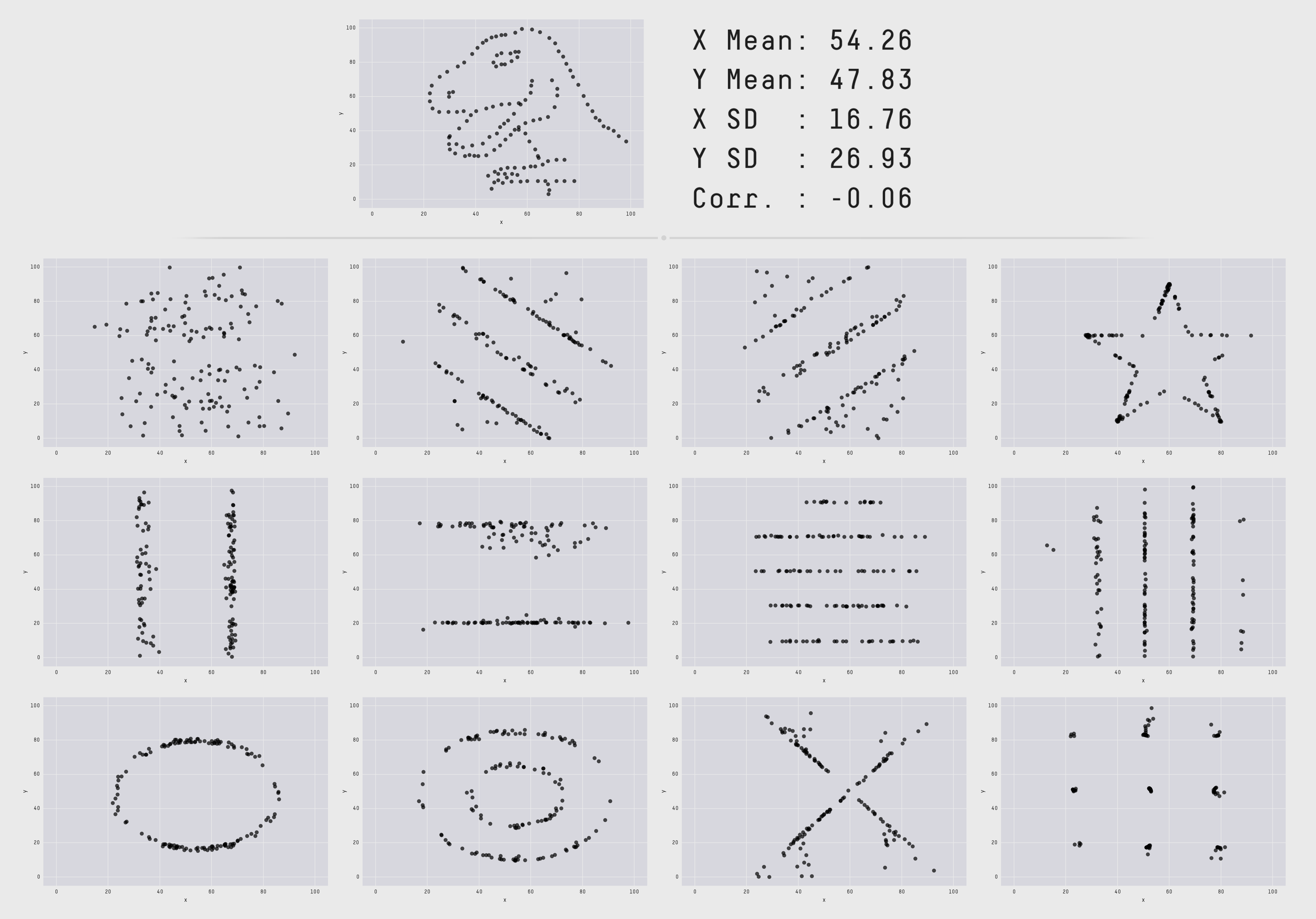
Anscombe’s quartet is a collection of four data sets of points in the plane. When graphed the data sets are obviously very different, but they have identical sets of descriptive statistics. Newer variations on the same theme include the delightful Datasaurus dozen, which includes animations of deformations from one step into another where the descriptive statistics are kept identical during the animation.

I’ve seen Anscombe’s quartet cited in discussions around monitoring and observability to assert that the average and standard deviation (two of the statistical tools used in the quartet) are not useful for monitoring and alerting; instead one should use percentiles. I agree with the conclusion but think it does not follow from the premise, and would like to offer some thoughts on the theme from the perspective of a reformed geometer.

To do so, I’d like to work out some examples involving the average and standard deviation. The data sets above involve collections of points in the plane but I’d like us to discuss data modeled on timeseries instead. The difference isn’t important, everything we say applies to both theaters, but the geometry we want to point out is easier to see in the latter.

The trolley problem asks how to decide between the lives of people in two groups. At the moment, it comes up in our industry in discussions around self-driving cars: Suppose a car gets into a situation where it must risk injuring either its passengers or pedestrians; which ones should it prioritize saving?

Always choosing one group leads to suboptimal outcomes. If we always save the pedestrians, they may perform attacks on car riders by willfully stepping into traffic. If we always save the passengers, we may run over a pedestrian whose life happens to be of greater worth than that of the passengers.

The crux of the trolley problem is how we should make the choice of what lives to save. As with all hard problems without clear metrics for success, it’s best to solve this by having the participants decide this for themselves.

Every time we view a website, our friendly ad networks must decide what ads we should see. This is done by having our user profile put up on auction for prospective advertisers. During a handful of milliseconds, participants may inspect our profile and place a bid for our attention according to what they see.

The same technology could be trivially repurposed for deciding the trolley problem in the context of self-driving cars.

Assume the identity of every participant in the trolley scenario is known. Practically, we know the identity of the passengers; that of the pedestrians could be known if their phones broadcast a special short-range identification signal. An incentive for broadcasting such a signal could be that we would have to assume that a person without one were one of no means.

Given this information, a car about to be involved in a collision could take a few milliseconds to send the identities of the people involved to an auction service. Participants who had the foresight of purchasing accident insurance would have agents bidding on their behalf. The winner of the bid would be safe from the forthcoming accident, and their insurance would pay some sum to the car manufacturer post-hoc as a reward for conforming to the rules.

The greater a person’s individual wealth, the better insurance coverage and latencies they could purchase, and the more accidents they could expect to survive. This aligns nicely with the values of societies like the United States, where the worth of a person’s life is proportional to their wealth.

As this system lets self-driving car manufacturers off the hook for any decisions taken, and would need coordinated ethical action on the behalf of software engineers to not be implemented, we expect to see this system in action in the world in short order.

I’m pleased to announce the release of my new card-drawing game Infosec.

The rules of the game are simple. It is for two or more players. The player with the fewest friends is the Infosec Expert; the other players are the Coworkers.

To start, the Infosec Expert deals three cards face down from a standard deck of cards. The Coworker on the Infosec Expert’s right hand should draw one card.

"Which card?" the Coworker may ask.

"This is a simple phishing exercise," the Infosec Expert should reply. "Just pick a card."

"But they all look the same," the Coworker may object.

"Draw one. And get it right."

This exchange should go on in increasingly hostile tones until the Coworker agrees to draw a card. It will have been the wrong card. The Infosec Expert should inform the Coworker:

"You got phished. You moron. You fucking idiot. You’re such a goddamn waste of space and time. How could you have gotten this so wrong? Were you even trying? Answer me. What the fuck was that?"

Feel free to ad-lib along these lines, or draw as many cards as you want from the accompanying Admonishment Deck (expansion packs available). Include ad-hominem attacks and use as many personal details as you know. Interrupt the Coworker if they try to reply. Don’t hold back.

Once the Coworker is silent, the Infosec Expert should collect the cards, deal new ones, and proceed to the next Coworker in line.

The game ends with the Infosec Expert’s victory when all the Coworkers have left.

Like so many things I’m supposed to do but don’t — getting exercise, eating right, sleeping well, standing up for women and minorities in public spaces — backing up my data has always been something I’ve half-assed at best.

I’ve lugged around an external hard drive with a few hundred gigabytes of data for the last 10 years, and made backups to it once every three or four years or so. Every time I’ve tried restoring anything from those backups I’ve regretted it, because of course I just bought the drive, plugged it in and copied stuff to it, so it is a FAT32 drive while I have mostly had EXT4 filesystems, which means all my file permissions get lost during the process.

I’ve written shameful little shell scripts to set file permissions to 0644 and directory permissions to 0755, recursively, many many times.

Part of my problem was that I both know just enough rsync to be dangerous and have a credit card so I can provision cloud VMs, so forever just around the corner was my perfect backup solution that I’d write myself and maintain and actually do instead of dealing with whatever I had going on in my life. I’ve come to accept that this will never happen, or perhaps more definitively, that I’d rather cut myself than write and maintain another piece of ad-hoc software for myself.

Luckily I recently found two things that have solved this whole problem for me: borg and rsync.net.

Borg is backup software. It compresses and deduplicates data at the block level, and strongly encourages (but does not force) you to encrypt data before backing it up. It is everything I’d want from my half-assed rsync and shell script abomination.

I read its documentation a couple of times and was impressed. I then set about comparing different VM hosts to see which one would give me the cheapest block storage option, when the result of some random google search led me to rsync.net. They are a company that stores backups, pretty cheaply, and even more cheaply if you use borg to take them. I guess they just really love borg and want us to love it too.

I signed up for their cheapest plan, which starts at 100GB stored for $18 per year. They have no network in- or egress costs, and the storage amount can be adjusted at any time. Once my account had been activated, I did a little password reset dance, and uploaded a public SSH key.

I wanted to back up my $HOME directory, so after installing borg I ran:

This created a remote borg repository called "home" on rsync.net’s servers. The environment variable is so we use a more recent version of borg on the remote server (version 1.1.11 at the time of writing), as the default version is rather old (version 0.29.0).

When choosing what encryption method to use, one can choose between a "repokey" or a "keyfile". They both create a private key locked with a passphrase; the difference is that with "repokey" the key is stored in the borg repo, while with "keyfile" it is stored outside of it. This boils down to whether we think a passphrase is enough security for our data, or whether we think having a secret keyfile is necessary. I figured my password manager could create a strong enough passphrase for my needs, and I didn’t want to think about losing the keyfile, so I chose "repokey-blake2".

To create my first backup, I ran

which created the archive "backup-1" in my "home" borg repository. I didn’t change the compression algorithm from the default one.

By default borg compresses data with lz4. It can use other compression methods (xz, zlib, zstd). I compared their compression ratios on some binary files I had and found no difference between them. I think this is because the large binary files I have are mostly audio and video files in lossy formats, which don’t seem to benefit very much from further compression. I have a lot of text files as well, but text takes up so little relative space on today’s hardware that it makes no sense to spend CPU cycles on compressing it better than lz4 does.

This backup command hummed along for a good while, and through a couple of reboot cycles. Doing a second backup right after it finished (or the day after) took a lot less time because of the deduplication:

Restoring from backup is also easy:

I set this up to run as a daily timed systemd service at noon (very easy on NixOS, which every Linux user should be using unless they hate themselves), and will never, ever think about this again. For a handful of bucks a year, that is a good deal.

A common theme among the people who fall in love with Nix (or its cousin NixOS) is that they want it to manage everything for them. Finding out the limits of that capability and where it breaks down is part of each’s journey.

An obvious enough limit to Nix’s reach is secret management. It can easily handle public keys, SSH or cryptographic ones, but the private keys cannot be managed by its store as it is readable by all.

The promise of Nix is that we will never break our system by updating it. We can always roll back to a previous working version, once we have a working version at all. This is in contrast to, say, every other Linux distribution. I have borked Ubuntu, Arch, Fedora and others during system updates. Often the safest way to update the system is to back up /home and reinstall the OS.

From somewhere comes the idea that a user on a Linux system should be able to install their own programs and manage their own system services. (See Chris Wellons for where you can run with this idea to if your sysadmin gives you a C compiler.) This seems odd from a historical perspective. In a true multi-user system, the system administrators normally do not want users to be able to install arbitrary software or run services. On a modern "multi"-user system, where there is a only single user, avoiding system packages and services seems like some kind of theater.

Yet we do it anyway. An argument I sometimes make to myself is that this is a cleaner separation between what I need the system to do versus what I do on it. I may want to be able to run traceroute as root, but I don’t care about root being able to run the Go compiler.

NixOS has facilities to enforce this separation. It happily creates users and their home directories, and can fill in some of the bits that go there, like public SSH keys. It can install packages for specific users, and allow them to define systemd services. It will not manage the configuration of specific user packages (like dotfiles) without some coercing. One can presumably create custom derivations of, say, ZSH with all the configuration one wants, but who has the time?

Home manager wants to fill this gap and bring the power of Nix to user environment and configuration management. It lets individual users say what packages they want installed; what services they want run; and what configuration files should go where. On the surface it seems like something I should love, but after using it for a month I wrote it out of my system and now use plain NixOS.

I used Home manager for three things:

The first one was never a big attraction. Home manager lets us define a list of packages in home.packages of packages to install. If we control the system configuration, we can acheive the same by defining those packages in users.users.$username.packages.

If a user controls the system configuration (directly or through a sysadmin), they can also define their own user services via systemd.user. Home manager’s selling point is that it comes with a large list of already defined services that we can enable with a boolean flag, instead of having to write our own service configuration. This is admittedly nice. In the end, I found that learning the idiosyncrazies of each home manager service definition was a less useful use of my time than learning how to define NixOS systemd services once and for all. The latter is after all where the former end up.

As a long-time sufferer of dotfile management, I had high hopes for the third point. And indeed, home manager will manage dotfiles just fine. It can do this in two modes: it can generate a config file from various options we fill out if someone has written a home manager module for the program we’re trying to configure, or it can plomp a file on the system verbatim from a source. I used the latter, as I didn’t feel like learning a configuration language to be able to partially configure program dotfiles was a good idea.

This works well, until we want to change anything in a dotfile. This experiment with home manager coincided with a regular low point in my life in which I try to use emacs. This comes with quite a lot of .emacs changes as I use Lisp for the only thing it’s ever been good for; configuring a text editor in the most complicated way imaginable. Now, the dotfiles that home manager (or Nix) puts on our systems are read-only, so every change would involve changing the source file and running home-manager switch. This seems like unnecessarily many steps, especially after I saw this brilliant Hacker news comment, which after a week of use is a much better solution for this problem.

All in all home manager is nice software. I can see it being useful for people who either don’t control the system they run on but want to use Nix in user mode to run their corner of it, or for those Nix users who gamers (a well-adjusted group of humans if there ever was one) would call "filthy casuals", that is, people who just want things to work and don’t care very much about learning how to write enough Nix to make that happen.

I’m not included in those groups, as I run this system and explicitly want to learn to use Nix in anger so I can try and fail to convince people to run it in production at work. Home manager is fine software and if it makes you happy, then please use it.